EXPLAIN ANALYZE: Reading a Plan Line by Line

When a query is slow, the plan tells you why. A plan is the tree of steps PostgreSQL chose to produce the answer. EXPLAIN shows the plan it would use. EXPLAIN ANALYZE runs the query and shows what really happened, next to what PostgreSQL expected to happen. The Intermediate course read a short plan to decide on an index. This lesson reads a longer one line by line, because the slow step is rarely the first line you see.

The shop is too small for a plan to mean much, so this lesson builds a table of 20,000 invented orders with generate_series. The values come from arithmetic, not from random(), so every run gives the same data.

A table big enough to matter

CREATE TABLE big_orders AS
SELECT g                                AS order_id,
       (g % 8) + 1                      AS customer_id,
       DATE '2026-01-01' + (g % 365)    AS order_date,
       CASE WHEN g % 100 = 0 THEN 'cancelled'
            WHEN g % 100 < 4 THEN 'new'
            WHEN g % 100 < 12 THEN 'paid'
            ELSE 'shipped' END          AS status,
       ((g % 97) + 0.5)::numeric(8,2)   AS total
FROM generate_series(1, 20000) AS g;
ALTER TABLE big_orders ADD PRIMARY KEY (order_id);
ANALYZE big_orders;
ANALYZE customers;
SET max_parallel_workers_per_gather = 0;

SELECT 20000
ALTER TABLE
ANALYZE
ANALYZE
SET

Most orders are shipped. Only 8 in every 100 are paid, and 3 in every 100 are new. The ANALYZE lines gather the statistics the planner reads, and the SET turns parallel workers off for this session so the plan has the same shape on every machine.

Read the plan from the inside out

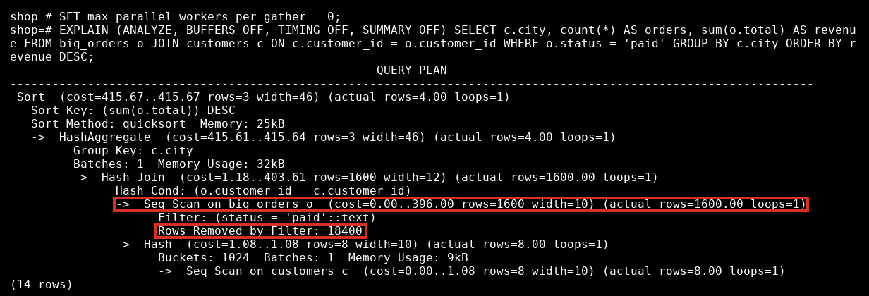
This query asks for revenue per city for paid orders, biggest first. Run it with EXPLAIN ANALYZE. Two options keep the output repeatable: TIMING OFF and SUMMARY OFF remove the clock readings, and BUFFERS OFF removes the cache counters that PostgreSQL 18 prints by default.

EXPLAIN (ANALYZE, BUFFERS OFF, TIMING OFF, SUMMARY OFF)
SELECT c.city, count(*) AS orders, sum(o.total) AS revenue
FROM big_orders o
JOIN customers c ON c.customer_id = o.customer_id
WHERE o.status = 'paid'
GROUP BY c.city
ORDER BY revenue DESC;

                                                    QUERY PLAN
------------------------------------------------------------------------------------------------------------------
 Sort  (cost=461.67..461.67 rows=3 width=46) (actual rows=4.00 loops=1)
   Sort Key: (sum(o.total)) DESC
   Sort Method: quicksort  Memory: 25kB
   ->  HashAggregate  (cost=461.61..461.64 rows=3 width=46) (actual rows=4.00 loops=1)
         Group Key: c.city
         Batches: 1  Memory Usage: 32kB
         ->  Hash Join  (cost=1.18..449.61 rows=1600 width=12) (actual rows=1600.00 loops=1)
               Hash Cond: (o.customer_id = c.customer_id)
               ->  Seq Scan on big_orders o  (cost=0.00..442.00 rows=1600 width=10) (actual rows=1600.00 loops=1)
                     Filter: (status = 'paid'::text)
                     Rows Removed by Filter: 18400
               ->  Hash  (cost=1.08..1.08 rows=8 width=10) (actual rows=8.00 loops=1)
                     Buckets: 1024  Batches: 1  Memory Usage: 9kB
                     ->  Seq Scan on customers c  (cost=0.00..1.08 rows=8 width=10) (actual rows=8.00 loops=1)
(14 rows)

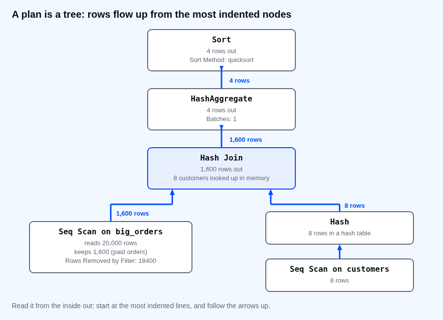
Indentation is the tree, and each -> is a child node. Rows flow upward: a node asks the nodes under it for rows and passes its own result to the node above. So start at the most indented lines and read upward.

• Seq Scan on big_orders. It read the table from start to end and kept the rows that passed the filter. Rows Removed by Filter: 18400 is how many it read and threw away. The 1,600 rows it kept are 8% of 20,000.
• Seq Scan on customers, then Hash. The 8 customers were put into an in-memory hash table.
• Hash Join. Each paid order looks up its customer in that hash table. The join keeps all 1,600 rows because every order has a customer.
• HashAggregate. It groups the 1,600 rows by city. Batches: 1 means the groups fit in memory. A higher number means the step spilled to disk, which is slower.
• Sort. It orders the 4 city rows. Sort Method: quicksort means it sorted in memory. You would see external merge Disk: if it did not fit in work_mem.

Each node shows two groups in brackets. The first, cost=0.00..442.00 rows=1600 width=10, is the plan: the startup cost and total cost in arbitrary units, the number of rows PostgreSQL expects, and the average row width in bytes. The second, actual rows=1600.00 loops=1, is what happened. Costs are not seconds. Use them to compare two plans of the same query, not to predict time.

Estimated rows against actual rows

The most useful habit is to compare rows= (expected) with actual rows= (real) on every node. Here the scans and the join match (1,600 and 8). The group count is 3 against 4, a small miss that does not change the plan. When they are far apart, the planner chose the plan on wrong information. A join method that suits 10 rows can be a disaster for 100,000, and the next lesson explains where those wrong guesses come from.

Loops: a node that runs more than once

Some nodes run once for every row that the node above hands them. loops tells you how many times, and actual rows is the average per loop, not the total. Multiply them to get the total. Here is a query that counts the orders of each customer with a subquery in the SELECT list.

EXPLAIN (ANALYZE, BUFFERS OFF, TIMING OFF, SUMMARY OFF)
SELECT c.name,
       (SELECT count(*) FROM big_orders o WHERE o.customer_id = c.customer_id) AS orders
FROM customers c;

                                                 QUERY PLAN
-------------------------------------------------------------------------------------------------------------
 Seq Scan on customers c  (cost=0.00..3587.16 rows=8 width=17) (actual rows=8.00 loops=1)
   SubPlan 1
     ->  Aggregate  (cost=448.25..448.26 rows=1 width=8) (actual rows=1.00 loops=8)
           ->  Seq Scan on big_orders o  (cost=0.00..442.00 rows=2500 width=0) (actual rows=2500.00 loops=8)
                 Filter: (customer_id = c.customer_id)
                 Rows Removed by Filter: 17500
(6 rows)

The subquery is the SubPlan 1 node. It runs once for each of the 8 customers, so it shows loops=8. Look at the Seq Scan on big_orders under it: actual rows=2500.00 loops=8 and Rows Removed by Filter: 17500. Both numbers are per loop. Over the 8 loops PostgreSQL read the whole 20,000-row table 8 times, and threw away 140,000 rows to keep 20,000. On 8 customers that is nothing. On 80,000 customers it is the reason the report never finishes.

A node with a small actual rows and a large loops is a common hidden cost: each loop is cheap, and there are thousands of them. Joining the two tables and grouping gives the same answer with one pass over the big table, and an index on customer_id is the other way out. The next lessons cover both the estimates and the indexes.

EXPLAIN ANALYZE really runs the statement

BEGIN;
EXPLAIN (ANALYZE, BUFFERS OFF, COSTS OFF, TIMING OFF, SUMMARY OFF)
DELETE FROM big_orders WHERE status = 'cancelled';
ROLLBACK;
SELECT count(*) AS cancelled_left FROM big_orders WHERE status = 'cancelled';

BEGIN
                        QUERY PLAN
-----------------------------------------------------------
 Delete on big_orders (actual rows=0.00 loops=1)
   ->  Seq Scan on big_orders (actual rows=200.00 loops=1)
         Filter: (status = 'cancelled'::text)
         Rows Removed by Filter: 19800
(4 rows)

ROLLBACK
 cancelled_left
----------------
            200
(1 row)

The plan shows the delete reading 200 rows, and the ROLLBACK put them back.

Common mistakes

• Reading the plan from the top instead of from the most indented nodes.
• Treating cost as time.
• Ignoring loops and comparing a per-loop row count to the estimate.
• Checking only the total time and not the node where the estimate is far from the actual rows.
• Running EXPLAIN ANALYZE on a data-changing statement outside a transaction.

If you skip this, you will tune by guessing: add an index, run it again, and hope. Which node of the slowest query in your own system has the biggest gap between the estimate and the actual rows?